Kyle R. Chickering

The goal of this project is to estimate the best possible count of the detected objects per vine given a series of images together with GPS image and plant locations.

Data Inspection

We are given the following data sources:

Fundamentally we can distill this conceptually into a bunch of images with bounding boxes and geolocation data.

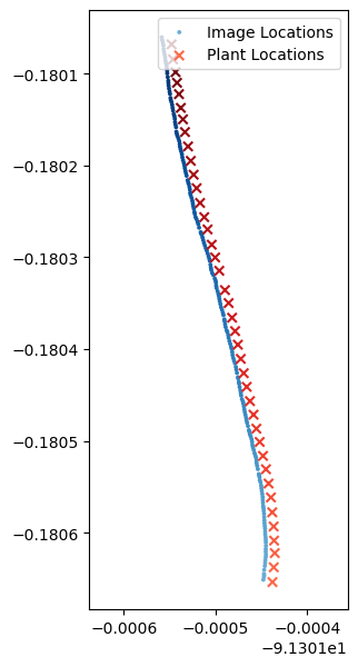
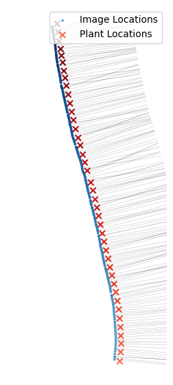
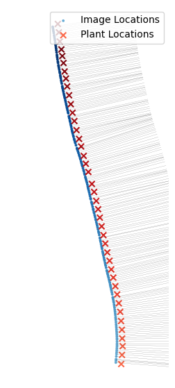
A perusal of the data quickly reveals that the vehicle is moving North-West, taking photos to its right. This is best observed by plotting the geo-location data through time. On the left we have plotted the image locations and the vine locations increasing in darkness over time. On the right we have plotted the (very downsampled) images as a gif showing roughly what the computer “sees”, which is the images and the bounding boxes.

Our main concern here is that that there is a lot of lens distortion. We are going to have to address this later (foreshadowing).

Naïve Solution

If we squint at the task we can implement a pretty simple solution. We first estimate how many times each object is “duplicated”, then estimate how many images there are of each vine, and use these values to do a moving average over the image.

Originally I guessed that there was one duplicate per object, but after working with this dataset some more I think that there are actually fewer duplicates than I had originally though. It seems safe to assume that on average there is less than one duplicate per object.

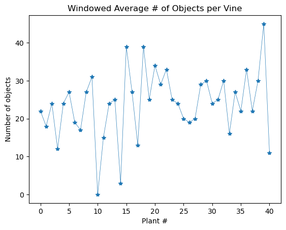
If we compute $\#\text{ Images } / \#\text{ Vines }$ we get 4.83 images per vine. Using these two metrics we load our data into Pandas and can implement the following extremely simple solution

lens.groupby(lens.index // 4.83).sum().plot(marker='*', linewidth=0.5)
plt.xlabel('Plant #')
plt.ylabel('Number of objects')
plt.title('Windowed Average # of objects per Vine')
plt.show()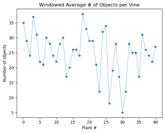

At first I thought that this was too many objects per vine, but doing a rough spot check of the data indicates that, while it is often an incorrect count, my naïve estimate isn’t wildly off.

Spatial Localization of Objects

Our naïve solution is simple, but does not actually use all of the data that we are given. In other-words we are not maximizing the given information. In particular we have not used any of the geo-location data, which can be used to more reliably resolve object locations. Since the density of the vines, the spacing of the vines, and the speed of the vehicle are not constants, we expect that our solution above does not accurately capture the objects per-vine.

We propose and implement a more sophisticated algorithm which uses the geo-location data to resolve the object locations in 3D, and associate them with specific vines.

Outline of Proposed Solution

Imagine our vehicle driving through the vineyard. For the sake of concreteness imagine an ATV with cameras fixed to it. As the vehicle drives, it traces out a continuous trajectory through space. We call this trajectory $\bm{x}(t)$ and consider $\bm{x}\in \R^2$ to be the $(x, y)$ coordinates of the vehicle at time $t$. Every time the camera takes a photo it records a sample of $\bm{x}(t)$. Thus, for our $N$ images we have $N$ time-samples of the trajectory. If $T=\{\, t_1, t_2, \cdots, t_N\,\}$, then $\bm{x}(T)=\{\,\bm{x}(t_1), \bm{x}(t_2), \cdots, \bm{x}(T_N)\,\}$ are the locations that the images were taken.

Since the camera is fixed in place to the ATV, and we assume that the ATV itself is rigid, the photos are taken with a fixed angle relative to the normal vector of the trajectory, denoted $\bm{x}^\perp(t)$. Furthermore, we can imagine that the vines trace out a continuous curve $\Gamma(x, y)$ through $\R^2$, and therefore at each time $T$, $\bm{x}^\perp(T)$ should intersect $\Gamma$. Thus, we can “project” the images and the associated bounding box info onto the sheet generated by extending $\Gamma$ in the $z$-axis (see below).

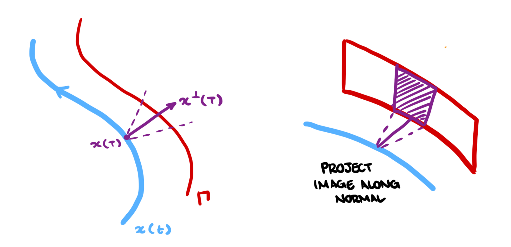
This scheme gives us a unified space to investigate object locations and the spatial relationships between the objects and the vines.

Practical Considerations and Implementation

This methodology, while great on paper, proves challenging to implement for several reasons. We discuss these reasons and our approach to solving them in what follows.

Difficulties

1. We have to account for lens distortion when localizing the objects.

2. The sampled trajectory is not very smooth, meaning that the normal vectors are not well aligned.

3. We must write code to project the object locations onto $\Gamma$.

4. We may have the same object represented multiple times.

5. At the end we must correlate each object with a given plant.

Dealing with Lens Distortion

This problem can be easily solved with OpenCV. I first built a widget that allows me to control the five lens distortion parameters and used this to find “good enough” distortion parameters for the camera. Since the images are all from a single, fixed camera, the distortion parameters should be constant throughout the entire process. I have included gifs of the before and after of my lens de-distortion.

Before

After

During this process I also use the distortion coefficients to “de-distort” the bounding boxes. Thus the de-distorted bounding boxes align with the objects in the undistorted images.

Computing the Normal Trajectory and Smoothed Normal Trajectory

When we compute the normals to the trajectory we use finite differencing, but due to the noisy-ish nature of the geo-location data, this gives noisy normals. To compensate for this we run a centered windowed averaging procedure to smooth out the normals. With more time we could run ablations to determine which window size is optimal for the downstream tasks, but for the purpose of this mini-project I determined that a window size of three was “good enough”.

Below I have plotted the original normals and two examples of smoothed normals. Observe that with a window size of 11 the normals are much less chaotic!

Original Normals

Averaged Normals: WS=3

Averaged Normals: WS=11

Spatially Locating the Objects: Part I

The first difficulty we have is determining the FOV of the camera, which we need to be able to determine where to project the objects. To do this I built another widget which allows me to adjust the FOV lines relative to the normal, given images of the vines. By correlating the images, FOV lines, normals, and geo-location data I was able to extract the camera FOV relatively easily

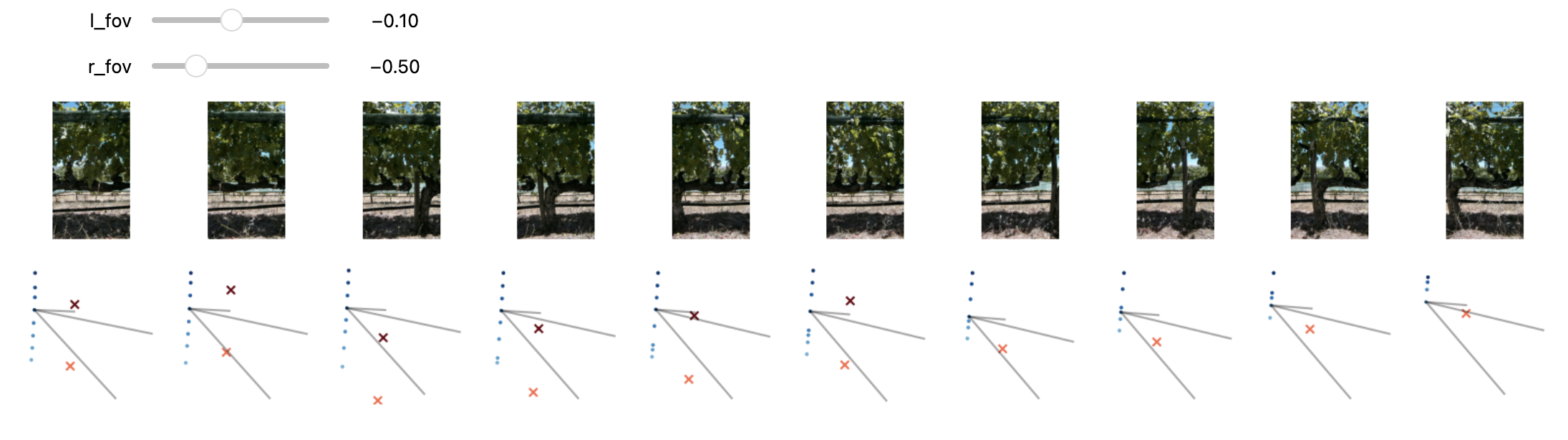
Once I have the FOV, I can then project the images onto any surface I like while retaining the correct proportions between the objects in the image.

Spatially Locating the Objects: Part II

Since the vine geo-location data is a lot less noisy than the normal vectors, I consider a “vine” as the line between adjacent plants. I also noticed that in this vineyard the plants are all bent to the right, and thus the “plant” can be considered the line moving in the negative $y$-axis from a given point towards the previous point.

Since I have a FOV, I can project the object coordinates onto the plane in 3D generated between these points using simple trigonometry, and then record the resulting intersection as the object’s actual location.

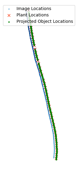
Below is an image of the image locations, plant locations, and the projected object locations. We see that my procedure projects the objects onto the plane formed by connecting the vine locations with lines.

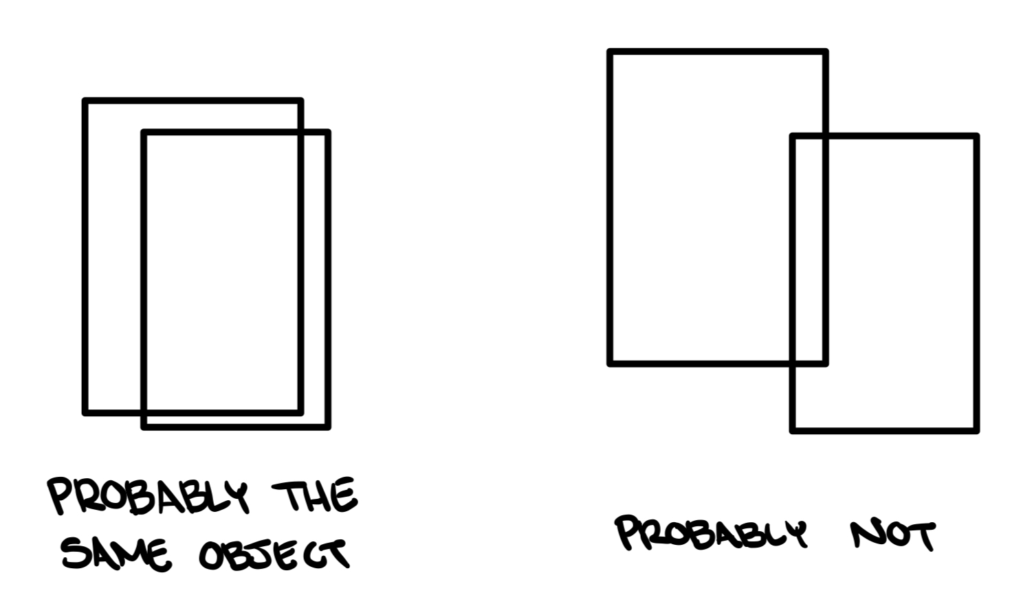
De-Duplication Procedure

This is also pretty straightforward. I iterate through all of the objects, and for each object I compare it’s location and size to the next $N$ objects. If I find a match I consider it a duplicate object and keep track of object “buckets”. The result of this procedure is a list of what my model believes to be “unique” objects.

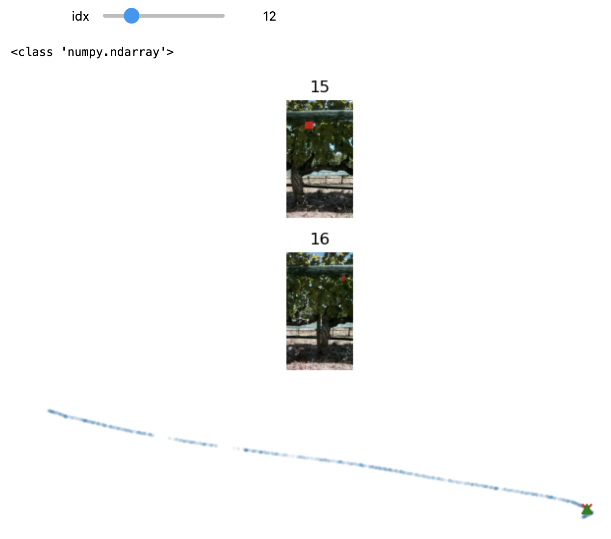
I introduce two hyper-parameters for the de-duplication process: an $(x, y)$ coordinate tolerance and a $z$ coordinate tolerance. These are “magic numbers”, and since the de-duplication process is pretty quick, I built another widget to tune the parameters (are you noticing that I like widgets?). There are other ways to do this, like using AoI between the boxes, these other methods might even be better, but in the absence of time I did not ablate this design choice.

And here is a look at this widget, which displays the duplicates as well as their spatial locations.

Associating Objects with Plants

The final step is resolving which objects belong to which vine. This is easy to do in the present context but I stress that my solution would not work in production.

Notice that the plants have (a) unique, increasing $y$ coordinate (b) are all “one-sided”. Thus, if an object’s $y$ coordinate falls into a certain range it is associated with a specific vine!

Results

How does this compare to our naïve method?

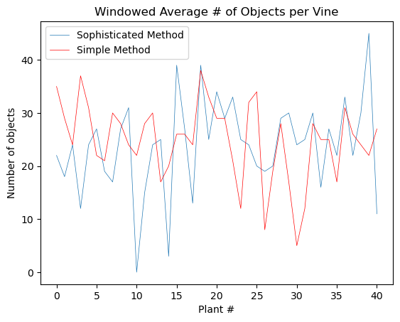
I have not done too much validation, but from the few samples I have looked at, my sophisticated method is much more accurate than the naïve method. There are a few failure cases that I would debug with more time, but for the time being I think that I am pretty happy with this solution.

Improvements and Further Steps

I am fully confident that with more time this algorithm can be made to be much more accurate. I believe that my method (both my methods) do not do an adequate job of identifying duplicated objects. With more time I could build some exploratory tools which allow us to get a better understanding of the characteristics that duplicated objects present, and building on this knowledge, develop a more sophisticated algorithm for identifying the duplicates.

It would probably take two or three hours, but it would be valuable for this dataset to get ground-truth human data to compare the quality of my model’s predictions. If this was ever going into production I would manually annotate several small datasets as ground truth (i.e. how many objects per vine). I would also spend more time building a human evaluation pipeline to quantify the quality of the model predictions.

Further Improvements

• Generalize all the steps to apply to other vineyard layouts since my method relies on the fact that we have a single line of vines.

• Python files instead of Jupyter Notebook hacking.

• Better human evaluation.