\(f:S^{d-1}\rightarrow \mathbb{R}_{\geq 0}\): a kernel density estimator given by
\(f(x)=\sum_{i=1}^N c_i K_t(x,x_i)\)
\(\mathcal{X}=\{x\in S^{d-1}: f(x)\neq 0\}\subset S^{d-1}\): domain on which \(f(x)\) is nonzero
\(\psi:\mathcal{X}\rightarrow \mathbb{R},\ \psi(x)=\log(f(x))\): the density estimator in log-coordinates
\(\mathcal{X}(a)=\{x\in \mathcal{X}: \psi(x)\geq a\}\): density super-level sets
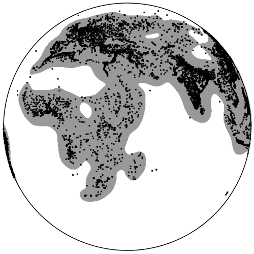
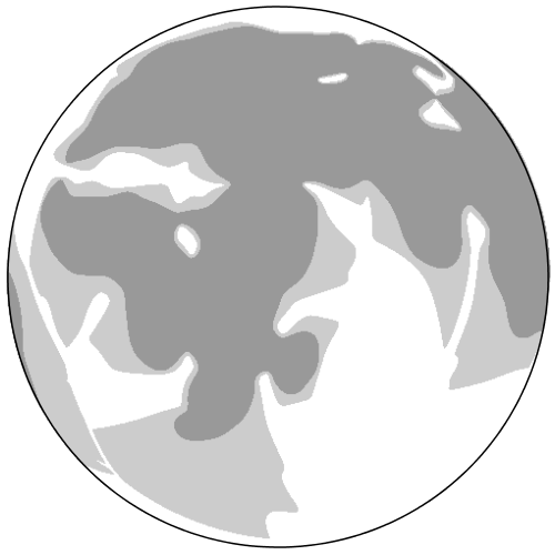
For instance, here is a plot of \(\mathcal{X}(a)\) on the globe for a list of the 10000 largest world cities, scale parameter \(t=500\), all \(c_i=.0001\), and a particular density cutoff value \(a=-7.77\):
Optimal transport map and the dual shape
Now, the terminology for the new concepts defined in the paper, following that of
Villani's well known book.
In this paper, we show that \(\psi\) is a \(c\)-convex function on the sphere, meaning that there exists a dual function
\(\psi^c:\mathcal{Y}\rightarrow \mathbb{R} \cup \{-\infty\}\) satisfying
\begin{equation}
\label{eq:psic}
\psi(x)=\sup_{y\in \mathcal{Y}} (\psi^c(y)-c(x,y))
\end{equation}
given by
\begin{equation}
\label{eq:psicdef}
\psi^c(y)=\inf_{x\in \mathcal{X}} (\psi(x)+c(x,y))
\end{equation}
for all \(x\in \mathcal{X}\). Note that we automatically have \(\psi^c\leq \psi\) by taking \(y=x\) in \eqref{eq:psicdef}.
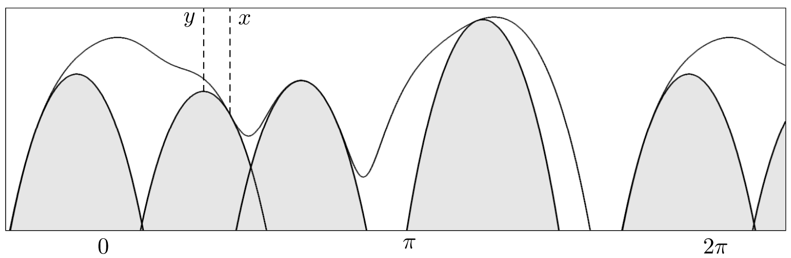
Here is an illustration of \(c\)-convexity in the one-dimensional case.
The top curve is a choice of \(\psi:S^1\rightarrow \mathbb{R} \cup \{-\infty\}\) based on 10 points. The meaning of \(c\)-convexity is that we can trace the graph of \(\psi\) from below by functions whose graph is of the form \(b-c_t(\_,y)\), which are the downwards facing parabola-like graphs in angular coordinates. The particular graph which contacts \(\psi\) at the point \(x\) is given by \(b=\psi^c(y)\), where \(y\) is the unique maximizer of the supremum in \eqref{eq:psic}. The graph of \(\psi^c\) is the curve traversed by the peaks as \(x\) moves around the circle.
As a result, we have three new objects:
\(T:\mathcal{X}\rightarrow \mathcal{Y}\) map which sends each \(x\) to the corresponding maximizer in \eqref{eq:psic}, i.e. the peak of the corresponding curve in the figure. It has an explicit formula in the paper, determined uniquely by fitting the curve to first order at \(x\).
\(\psi^c : \mathcal{Y}\rightarrow \mathbb{R} \cup \{-\infty\}\): the dual function defined above, which satisfies \(\psi^c(x)\leq \psi(x)\) for all \(x\).
\(\mathcal{Y}(a)=\{y\in \mathcal{Y}: \psi^c(y)\geq a\}\): the conjugate density super-level set, which satisfies \(\mathcal{Y}(a)\subset \mathcal{X}(a)\).
It is computationally difficult to evaluate \(\psi^c(y)\) at any given point
\(y\in \mathcal{Y}\), since it involves taking the infimum in \eqref{eq:psicdef}.
However, given \(x \in \mathcal{X}\), there is a closed formula for both
\(T(x)\) and \(\psi^c(T(x))\), determined by calculating the curve \(b-c(\_,y)\) which agrees with \(\psi\) to first order at \(x\), as in the figure. Therefore, while we can't evaluate \(\psi^c(y)\) directly for a given \(y\), we can sample points from
\(\mathcal{Y}(a)\) as follows:
Sample a point \(x\in \mathcal{X}\) from the underlying distribution of \(f\).
Simultaneously compute \(y=T(x)\) and \(b=\psi^c(y)\).
Accept \(y\) as a sample if \(b\geq a\)
It is not obvious, but this sampling scheme is stable with respect to isometric embeddings of \(\mathcal{D}\), such as adding extra coordinates of all zeros.
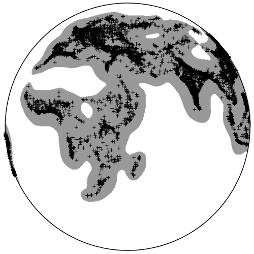
Here is the result of doing this for the above point cloud of world cities:
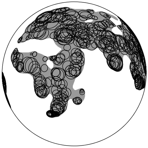
A direct consequence of \eqref{eq:psic} is that we may write \(\mathcal{X}(a)\) as the union of discs centered at the points of \(\mathcal{Y}(a)\):
\begin{equation}
\label{eq:union}
\mathcal{X}(a)=\bigcup_{y\in \mathcal{Y}(a)} \{x:c(x,y)\leq \psi^c(y)-a\}
\end{equation}
Plotting a random subsample of these discs, overlayed on \(\mathcal{X}(a)\) looks like this:
Statement and proof of the theorem
In the paper, we proved
Theorem We have
\(\psi\) is \(c\)-convex, and the transport map \(T:\mathcal{X}\rightarrow \mathcal{Y}\) has an explicit formula.
The dual shape \(\mathcal{Y}(a)\) is contained in the intersection of the linear span of \(\mathcal{D}\) with the sphere. The above contructions transform covariantly with respect to linear isometric embeddings.
The inclusion map \(\iota:\mathcal{Y}(a)\rightarrow \mathcal{X}(a)\) induces a homotopy inverse. It inverse can be represented by the restriction of \(T\) to \(\mathcal{X}(a)\).
The meaning of the second part is that the shape is that, unlike \(\mathcal{X}(a)\), \(\mathcal{Y}(a)\) is isometrically "stable" with respect to adding
new coordinates. This resolves a major issue with modeling \(\mathcal{X}(a)\) in higher dimension, which is that the \(\epsilon\)-covering of \(\mathcal{X}(a)\) grows exponentially with \(d\), even in the case of a single data point. This property is actually specific to this cost function, and would not be satisfied by other natural choices, such as taking a Gaussian along the tangent direction. On the other hand, the third item says that we lose no topological information by considering \(\mathcal{Y}(a)\) instead of \(\mathcal{X}(a)\).
The idea of the proof has a requires a similar trick as in the Gaussian case:
the most obvious method would be to use \(T\) to define a deformation retraction from \(\mathcal{X}(a)\) to \(\mathcal{Y}(a)\). The problem is that the restriction of \(T\) to \(\mathcal{X}(a)\) does not surject onto \(\mathcal{Y}(a)\), and also does not act on the identity on \(\mathcal{Y}(a)\), and so does not obviously determine a retraction. Moreover, since \(\psi^c\) does not have a closed formula, it is hard to imagine a way of modifying it.
Instead, remember that we have a closed formula for \(\psi^c(T(x))\), given by definition by \(\psi^c(T(x))=\psi(x)+c(x,T(x))\).
We may therefore consider a third space given by \(T^{-1}(\mathcal{Y}(a))\),
which contains both \(\mathcal{X}(a)\) and \(\mathcal{Y}(a)\). Here is what this set looks like:
We prove the third part of the theorem by showing that both \(\mathcal{X}(a)\) and \(\mathcal{Y}(a)\) are homotopy equivalent to \(T^{-1}(\mathcal{Y}(a))\), a key step being to determine a deformation retraction
from \(T^{-1}(\mathcal{Y}(a))\) to \(\mathcal{X}(a)\).
It turns out that this can be done using a straight-line homotopy, which moves along the arc connecting \(x\) to \(T(x)\) until coming in contact with the disc centered at \(T(x)\), as in the above figure.
Here is an illustration of this retraction:
In this figure:
The overall goal is to show that \(\mathcal{X}(a)\) (dark gray) is homotopy equivalent to \(\mathcal{Y}(a)\), which is not shown, but can be sampled from as above. Instead we show that both regions are homotopy equivalent to \(T^{-1}(\mathcal{Y}(a))\) (light gray). Showing that it is homotopy equivalent to \(\mathcal{Y}(a)\) is straightforward.
For the more difficult case, we picture a deformation retraction \(r: T^{-1}(\mathcal{Y}(a)) \times [0,1]\rightarrow T^{-1}(\mathcal{Y}(a))\) to \(\mathcal{X}(a)\) at several moving points
\(x \in T^{-1}(\mathcal{Y}(a))\)
which are the solid dots.
Whenever \(x\) is in the light gray region,
we have a nonempty disc centered at \(T(x)\), shown as a cross symbol. The disc is the one given by \eqref{eq:union}.
The deformation retract walks along the arc connecting \(x\) to its closest point in the disc.
The point of contact is shown as an open circle, which represents r(x,1).
When \(x\) is in \(\mathcal{X}(a)\), there is no line segment because \(x\) is already in the ball, and so is its own closest point. This satisfies one of the properties of a deformation retraction.
A key step involves showing that the path given by the line segment remains in the light gray region \(r(x,t) \in T^{-1}(\mathcal{Y}(a))\)