Accelerating PINN Experiments with -TangentProp - January 2025
Kyle R. Chickering - krchickering@ucdavis.edu
[ Homepage ]
This blog post accompanies this paper, these slides, and this GitHub repository. This blog post includes links to various sources, but the citation quality of this post is not commensurate with scientific standards. Please read the references in the paper for more formal citations.
In January of this year the world’s most famous mathematician, Terrence Tao, cited PINNs (Physics Informed Neural Networks) as a promising numerical method for assisting mathematicians in the search of a solution to the Navier-Stokes Millennium prize problem, which would garner the solver one million dollars!
The paper he cited (which can be found here) was also the motivation for the work we are discussing in this blog post. The authors use PINNs to find solutions to the Bousinesq equation, a complicated set of equations in self-similar coordinates. Their work is an important step in the quest to understanding how the solutions to fluid equations break-down in finite-time, and these types of solutions (nonlinear and nonlocal) are extremely difficult to compute using standard numerical methods (see for example this paper, which solves a similar problem using traditional numerics).
PINNs are neural networks (the “NN” in the name), which entails its own set of peculiarities when solving problems. The deep-learning revolution of the last decade has undeniably demonstrated the effectiveness of neural networks, but their use in numerical computation presents a tradeoff: we can compute interesting solutions at the cost of an enormous amount of computational power and time. The “neural network” portion of PINNs means that these methods are well suited to parallelization on GPUs, but the “physics informed” portion means these methods take an exponential amount of compute for higher-order equations (which we will discuss this below).
There are, in my view, three main impediments to mobilizing PINN techniques on an increasing number of problems
- Training PINNs is highly computationally inefficient. We discuss some of the reasons for this below.
- There is no rigorous error analysis for PINNs in general which makes assessing their accuracy difficult.
- PINN training is somehow unique in the neural network literature in that its training is highly unstable and we don’t have a clear sense of why (I am planning to write a blog post on this topic soon). Two recent results have begun the study of these instabilities, but much work remains to be done.
In this blog post (which is based on this paper which I wrote in December) we will present a technique for addressing the first point above: the computational inefficiency of training PINNs. In particular we propose an alternative algorithm to autograd which can compute the derivatives of a neural network (the “physics informed” part of PINN) in linear rather than exponential time. Due to the fact that most PINN applications take at least three derivatives, this reduction in asymptotic runtime yields significant speedups in end-to-end PINN training times.
Table of Contents
A Quick Primer on PINN Training
Deep Feed-Forward Neural Nets
The audience for this blog post may not be familiar with neural networks, and we give a quick overview of some basic concepts in neural network theory.
One of the reasons that we care so much about neural networks is that they are universal function approximators, meaning that for a given function and a desired precision there exists a sufficiently large neural network with weights such that the neural network approximates the function within that error tolerance.
Finding these weights is always theoretically possible, but can be practically difficult. In fact, many of the advances in neural networks and deep learning over the last few decades have been advances in training models.
We typically train neural networks using an optimization method called gradient descent. Gradient descent requires a supervised learning target, which means to train a network we must know the answer for a given set of inputs. Suppose that we have a set of pairs and a network which makes predictions. The learning target for such a neural network could be something like
which is the mean-squared error and is our loss function. Gradient descent updates the parameters of the neural network via the update rule
being a parameter which controls how large the weight updates are. This is an extremely simplified picture of training neural networks which we hope suffices for the purposes of this blog post.
PINNs
PINNs are neural networks which are trained to approximate the solution to a given ODE or PDE. Because neural networks with smooth activation functions are functional approximators, and functions are dense in the function spaces which we generally care about (think and Sobolev spaces), we can train a neural network using gradient descent to approximate the solution of the give differential equation.
Introductory literature abounds on the topic of PINNs and is easy to find online, and we concern ourselves here only with the highest-level details.
Let be a feed-forward, densely connected, neural network with parameters . Our goal is to optimize so that is a sufficiently good approximation to the solution of the differential equation . We train the neural network over the discrete domain using the loss target
which is the mean-squared error (MSE) of the differential equation residual , and where is an additional term which encodes the boundary conditions in the problem. Since is with a known derivative structure, we can exactly compute all of the derivatives appearing above in the loss function.
In theory, the approximation theorem ensures that we will converge to a good approximation of the (or a) true solution to given a neural network with sufficient capacity. In practice optimizing this loss function proves difficult due to a poorly conditioned Hessian, and there is no general theoretical error analysis available yet.
Training PINNs is further complicated by needing to enforce boundary conditions which serves to introduce problems typical of multi-target optimization. There are a slew of other practical problems that pop up and solutions to these problems are well studied in the literature (see our paper for further discussion).
We mention one more aspect of training PINNs which is relevant to the present discussion. Training a PINN based solely on the first-order loss target yields slow convergence in practice, often painfully slow. While the reasons for this are varied and only partially understood, it has been shown empirically that training convergence is greatly improved by replacing the first-order loss function with the higher-order Sobolev loss function
where the are relative weights and are treated as additional hyperparameters. What is important in the context of our present discussion is that the Sobolev loss function requires taking additional spatial derivatives during training.
PINNs: The Good and the Bad
PINNs occupy a somewhat strange place in the world of numerics. On the one hand, they allow for the computation of seemingly otherwise intractable numerical problems. On the other, they are slow to train, prone to poor convergence, and lack rigorous error analysis. These issues have raised concerns over the utility of PINNs as a numerical method, and I would venture to argue that for problems where traditional numerics already do a good job, PINNs are not worth pursuing except as an academic exercise.
However, a use case for which I feel PINNs are particularly suited is finding self-similar blowup profiles to challenging problems in fluids. Breakdown phenomena like shock formation can be understood as arising as a consequence of competing scalings between spatial and temporal features according to a prescribed power law. By converting into the coordinate system associated with these power law coordinates we can transform the shock formation process from a complicated nonlinear PDE to a much simpler nonlinear ODE.
This is the sort of problem that we mentioned in the introduction. These problems tend to be posed as boundary value problems with singular update rules. For example, the self-similar Burgers equation, written in it’s update form, reads
which is naïvely singular at the origin. This in itself is not insurmountable, however we also require to that we solve for and simultaneously. The constraint that we impose to find is a smoothness constraint on ; is smooth only for a countably infinite sequence of value for . I am not arguing that this task cannot be done using standard numerical methods, only that it is difficult to do so using current methodologies. PINNs allow us to have an exact form for an approximation of and thus solve for both and simultaneously using gradient descent on the target or the Sobolev target .
In summary, my belief is that PINNs are a niche numerical method which are impractical for many problems, and well-suited to a small number of problems.
Autodiff and -TangentProp
We assume that the reader has little to no familiarity with deep learning and neural networks, so we take a moment here to introduce the bare minimum on autodiff as well as give a brief historical perspective before diving into the technical details which motivate our research.
Autodiff
I would argue that the modern deep learning revolution would have been impossible without the introduction, implementation, and contemporary understanding of the autodifferentiation (autodiff) algorithm. Given a neural network with parameters which can be expressed as a directed acyclic graph (DAG), autodiff computes efficiently by running a forward pass through the DAG, storing the forward activation at each node, and then running a backwards pass through the same DAG and accumulating the gradients at each node. Since the optimization step for a neural network looks like
it becomes clear why the efficiency of autodiff fueled the deep learning revolution in the 2010’s: being able to compute these updates at scale allowed for the training of previously unthinkably large models. Since the last two decades have taught us that bigger models are usually better, autodiff can be seen as the héro des temps.
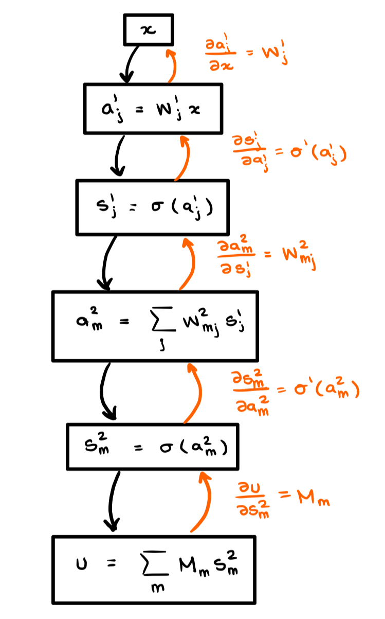
We begin with a high-level overview of autodiff, and then explain why this algorithm is poorly suited for the PINN use case. Fundamentally, autodiff works by representing every operation as a node in a directed acyclic computational graph (DAG) where each node has a forward operation and a derivative operation:
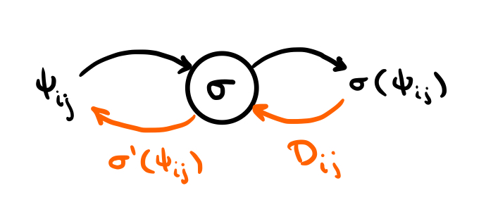
The figure above is the computational graph for the evaluation of the function . Thus, given the input , this computational graph represents computing the value . We compute this value by following the black arrows forward through the graph. At this node we also have a derivative operation, which is itself a node on a computational graph. Namely it is the operation where and are the node’s inputs and is the Hadamard (element-wise) product. For our simple example, , but for more complicated examples will be the value of the derivative of the upstream graph with respect to the current node. Thus, to compute the derivative for our forward operation, we follow the orange arrows backwards through the same graph.
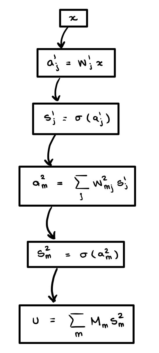
This example is, of course, too simple to be useful. We stress that power of computational graphs extends well beyond their usage in neural networks. For the purposes of this exposition we will use a simple two-layer neural network with an output projection layer to illustrate our ideas, however they will apply to neural networks of any size. Let , , , , and an activation function. Let be the corresponding neural network, that is
We can alternatively understand the network through the recursive formulas
This latter formulation makes drawing the computational graph quite easy!
On the left is the forward computation graph corresponding to the recursive definition for our neural network, and on the right is the same graph with the corresponding differentiation operations.
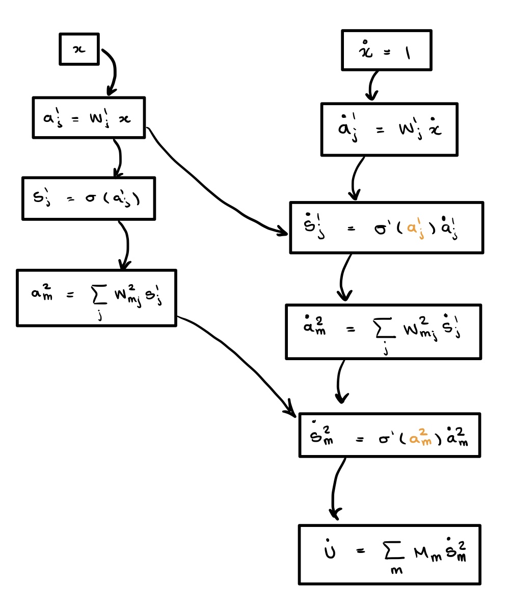
Autodiff then allows us to take this original graph and build a new computational graph for the derivative . We do this by tracing the derivative through the graph on the right! By the chain rule applied to we have
Where is the Hadamard (element-wise) product and is the standard dot-product. This same sequence of operations can be computed by following the orange lines up through the computational graph on the right. And here is the key: Doing this generates a new computational graph for the derivative! If we draw this new graph and it is immediately apparent that the functional composition introduces a new dependency which makes it so that we can no longer draw the graph as a simple “line” of nodes:
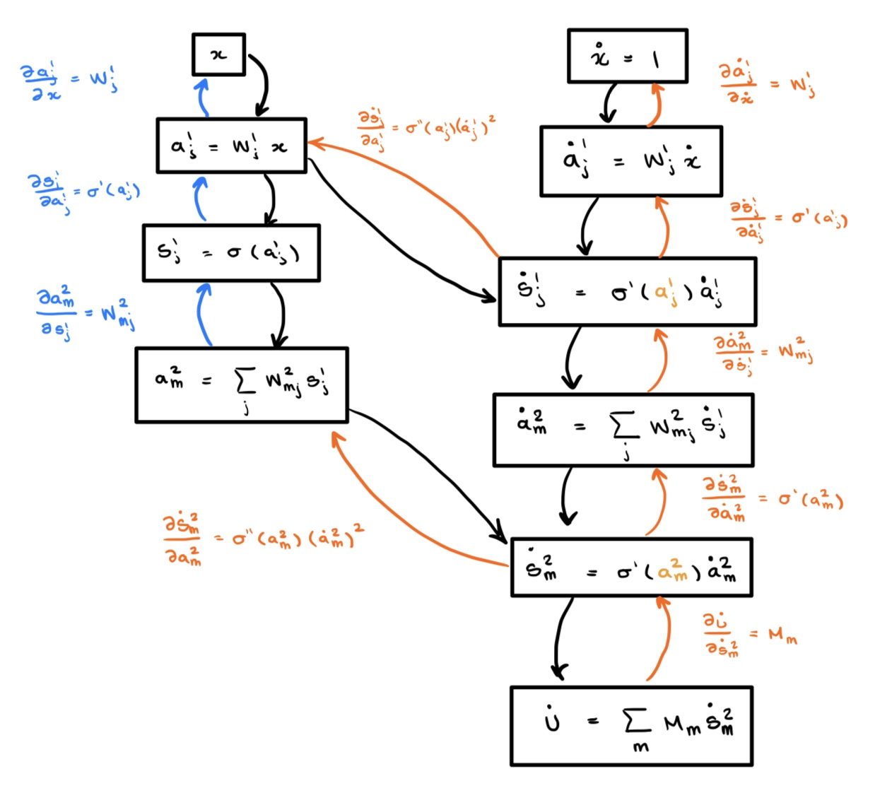
On the left is the computational graph for the first derivative, and to the right is the computational graph with the derivatives included. We note an important property, when we go to create the computational graph corresponding to the second derivative, the edges in blue will be computed twice, since they were already computed when we computed the forward pass for the zeroth derivative (our original graph). Note that this forward pass is required due to the nonlinear functional composition with : we need to compute the activations and to compute the derivative .
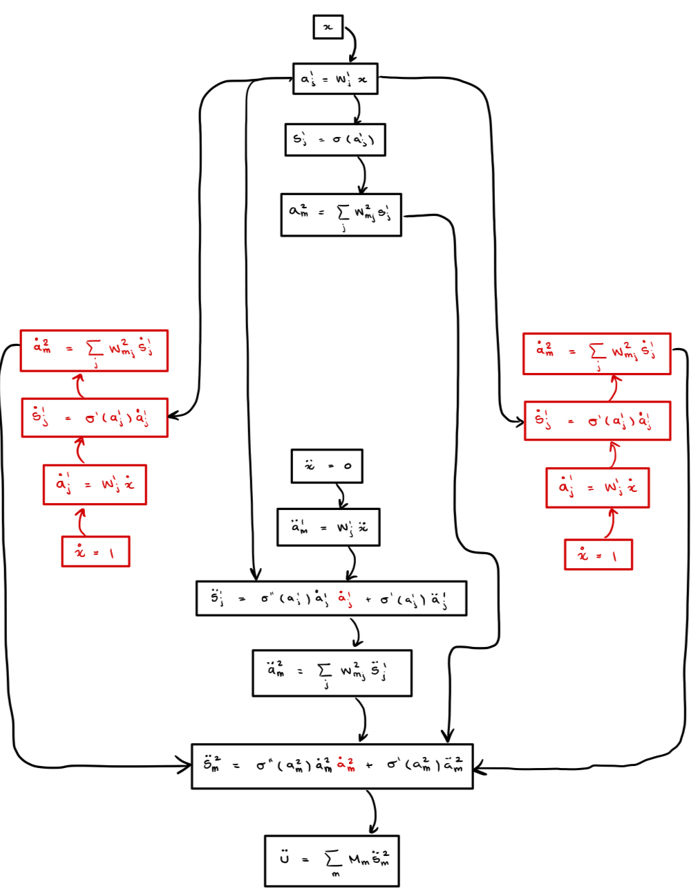
We present the computational graph for the second derivative and then cease our efforts in drawing these as they get increasingly complicated. Remember that you must resist the urge to draw the “correct” graph without the repeated computation, since the computer does not know that it already computed these values! We draw the re-computed values in red in the graph below.
Exponential Growth of Computational Graph of Derivatives:
Consider a neural network of depth . We notice from the above that the we can count the number of nodes by doubling all the nodes between the top order and bottom order derivatives. Thus we get the following sequence of node counts:
First:
Second:
Third:
That is, , where is the number of derivatives and hence the computational graph will grow like .
WARNING I: The actual computational graph computed by an autograd library will be much, much bigger, but this only changes the pre-factor. There are also graph optimizations that bring this runtime down a bit. I estimate that a good asymptotic bound is (see the figure below), which means the graph doesn’t actually fully double at each step.
WARNING II: The computational runtime to evaluate the graph will grow even faster, but still exponentially. This is because in our formulation the number of nodes does not necessarily scale linearly with FLOPs (see the note below on precise runtimes).
We can easily see this by simply plotting the number of nodes in a computational graph using a popular autodiff framework like PyTorch or Jax (see below).
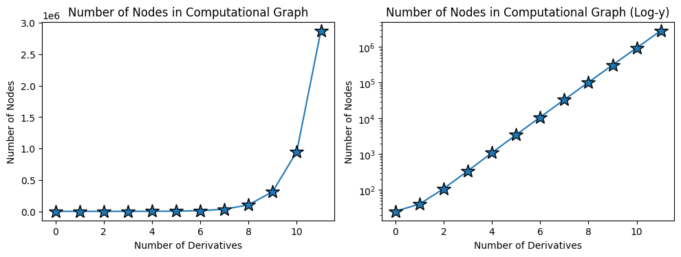
This figure shows empirically the exponential blowup in the size of the computational graph for a simple depth 3 neural network as a function of the number of derivatives we take.
And here is the main takeaway of why autodiff is the wrong tool for computing these derivatives (quickly):
Functional evaluation introduces extra dependencies in the computational graph of the derivative which result in additional computation needing to be done (recomputing derivatives). This leads to an exponential blowup in both memory and runtime when using autodiff to take high-order derivatives.
The TangentProp Formalism
For my generation of ML practitioners it is easy to forget that neural networks proceeded autodiff, and while the current era of deep learning is predicated on autodiff, there were almost 30 years of impressive neural network research prior to the introduction of autodiff.
It is easy to ignore the water you swim in, and it is hard to imagine that there are alternative methods to autodiff for computing derivatives! We will present a differentiation method which keeps track of repeated computation by unrolling the autograd graph and avoiding repeated computation, and was developed prior to the widespread adoption of autodiff.
We base our work off the TangentProp formalism introduced by Simard et al. in 1991. Written before the widespread adoption of autodiff in training neural networks, they propose a formalism for computing both and in a single forward pass. Rather than compute and evaluate the computation graphs using autograd, we can explicitly form a single computational graph since we know the explicit dependencies between derivatives. In particular, the activation at layer is given by
and we can directly differentiate this with respect to the network inputs to obtain
Note that as we compute nodes in the DAG, the activations for the neural network and its physical derivative at layer depend only on the activation (and its derivative) from the previous layer. Thus we can compute the physical derivatives in a single forward pass.
Our Approach: -TangentProp
The TangentProp paper computes a single derivative because for their use-case there was no reason to compute higher-order derivatives. However the principle that physical derivatives can be computed recursively, in a single forward pass, is not restricted to taking a single derivative. Thus, we propose -TangentProp, which extends TangentProp to multiple derivatives by computing in a single forward pass. Note that if we can accomplish this task we would obtain a runtime of , which beats the autodiff runtime of .
Most readers likely learned the Leibniz’s formula for taking higher-order derivatives of the product of two functions
where the constants are readily computable. Leibniz’s formula is the natural generalization of the product rule to higher dimensions, and Faà di Bruno’s formula is the lesser known generalization of the chain rule. In particular we have that
where the summation is taken over the set of partitions of , whereby is an -tuple satisfying . We denote , and note that is readily computable, albeit more complicated than the constants appearing in Leibniz’s formula.
Using Faà di Bruno’s formula it becomes clear how to extend to higher-order derivatives! Applying Faà di Bruno’s formula to gives
Thus, once implemented in code, we will be able to compute derivatives in (quasi)linear time. This implementation is not particularly difficult, and makes for a good exercise in a ML programming. We of course made several more advanced implementation choices, but at its core, the method is quite simple. We have our complete code posted on GitHub.
Finally, we leave the reader with the computational graphs for the second derivative computed via -TangentProp and ask that you compare this with the graph we drew for the second derivative above.
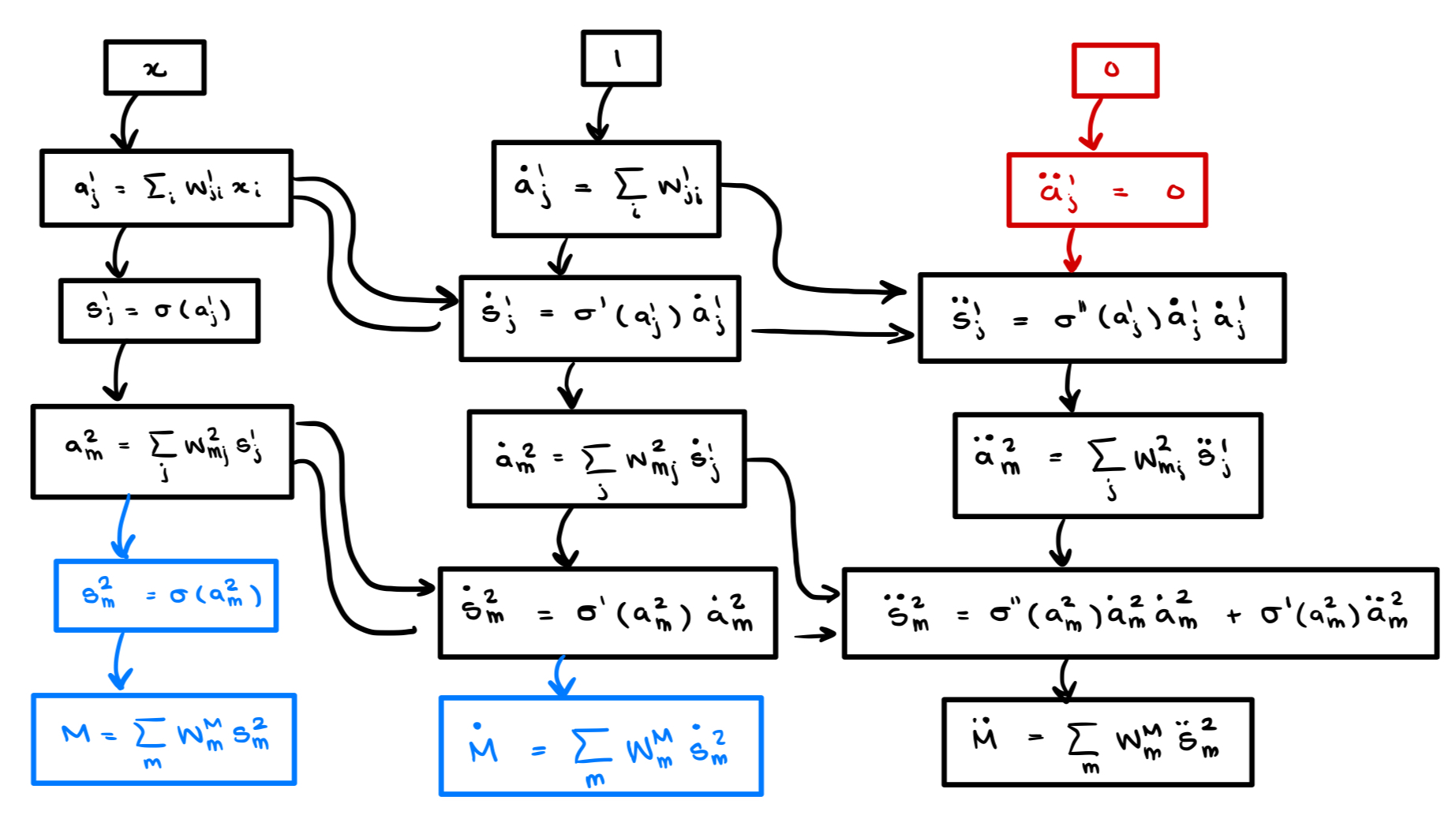
As you can see, nothing is repeated. We have managed to construct the “correct” computational graph instead of the complicated graph generated by autodiff.
While we did not implement these optimizations, we can see from the graph above that the upper portion of this computational graph (shown in red) can be pruned since the inputs will always be zero. Similarly, One can prune the columns of the lower portion (shown in blue) which correspond to unnecessary derivatives. However this pruning does not materially change the computation being done.
A Note on the Precise Asymptotic Runtimes of Autograd and -TangentProp
Our algorithm isn’t quite linear, and autograd isn’t quite exponential. -TangentProp is slightly super-linear (or sub-exponential), and autograd is slightly super-exponential. The reason is that the summation appearing above in Faà di Bruno’s formula introduces a non-trivial dependence on . Since the summation occurs over integer partitions of size , we must count the number of possible partitions. Luckily for us, this problem has interested combinatorialists for over a century, and they have introduced and studied the partion function defined via
The classical result of Hardy and Ramanujan provides a tight asymptotic bound for of the form
This root-exponential dependence on cannot be avoided by any differentiation algorithm, it is an unavoidable consequence of differentiation through function composition, which necessarily requires Faà di Bruno’s formula. Note than the the more exact runtimes for autodiff and -TangentProp are
respectively. Clearly for large the runtime of -TangentProp is faster. In particular autodiff is super-exponential and -TangentProp is sub-exponential (see the figure below).
.png)
Results
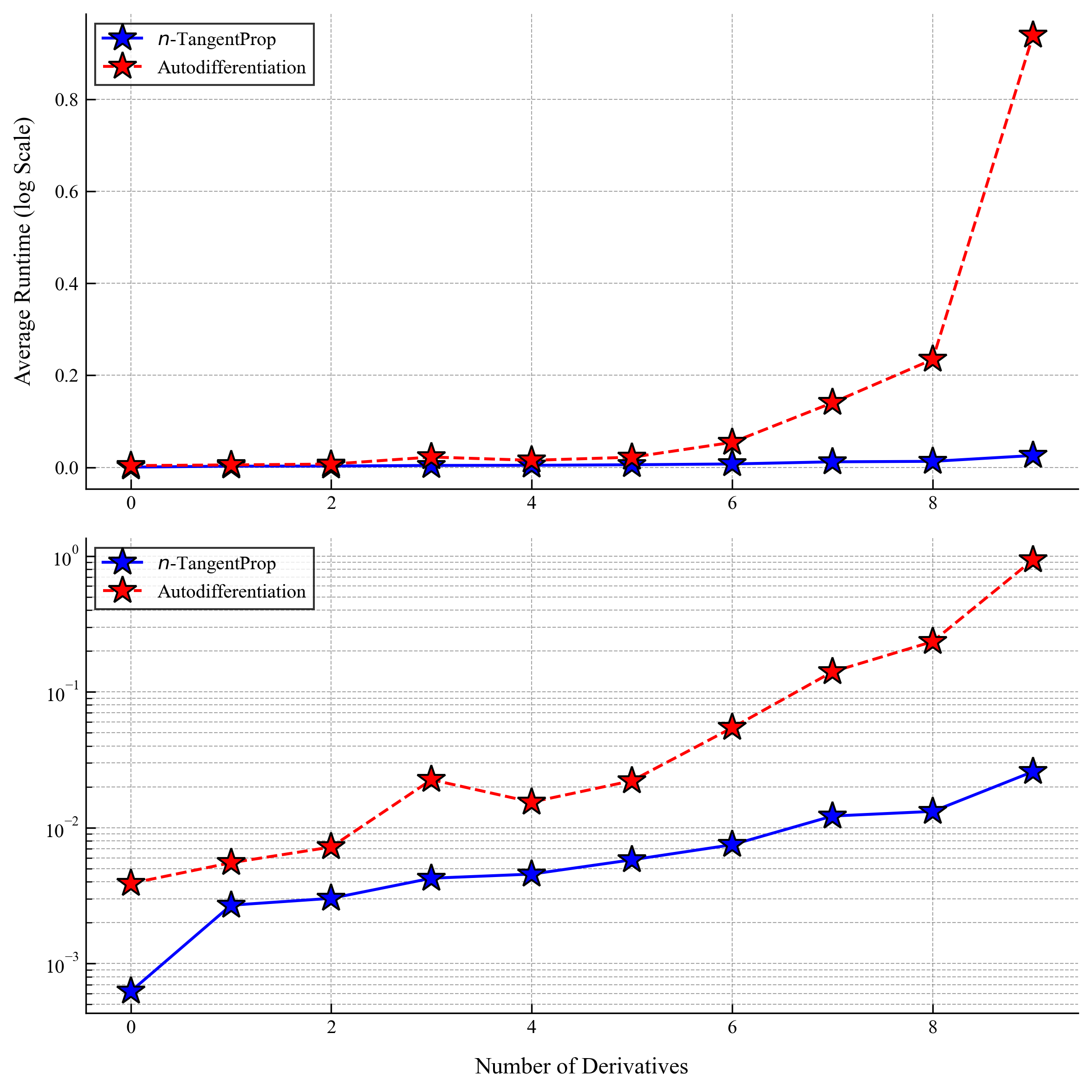
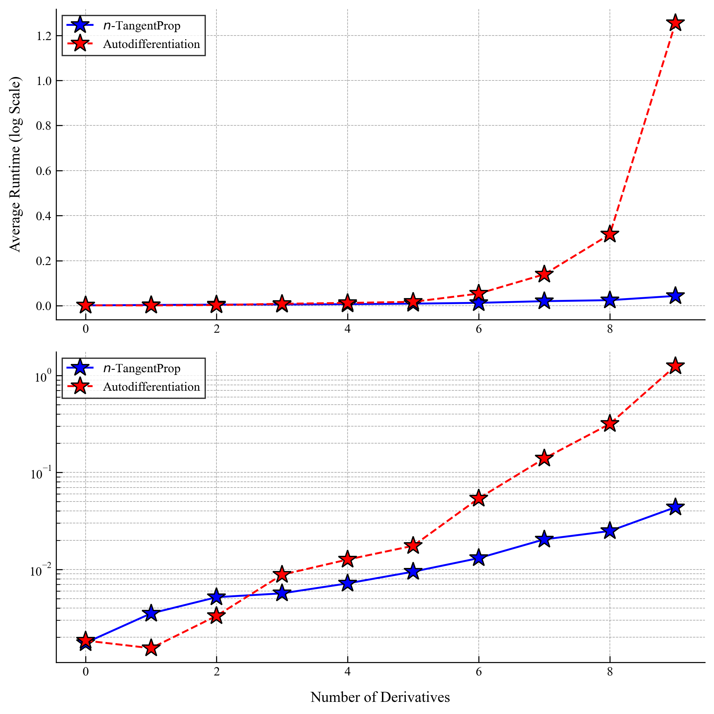
How much faster is -TangentProp than autodiff in practice? We ran several numerical experiments to quantify the performance increase with a special focus on computing the self-similar profiles for Burgers equation. The overarching finding is that, perhaps unsurprisingly, as the number of derivatives grows the exponential vs. linear scalings of these two methods begin to play a larger and larger role in the overall runtimes.
Results for General Neural Networks
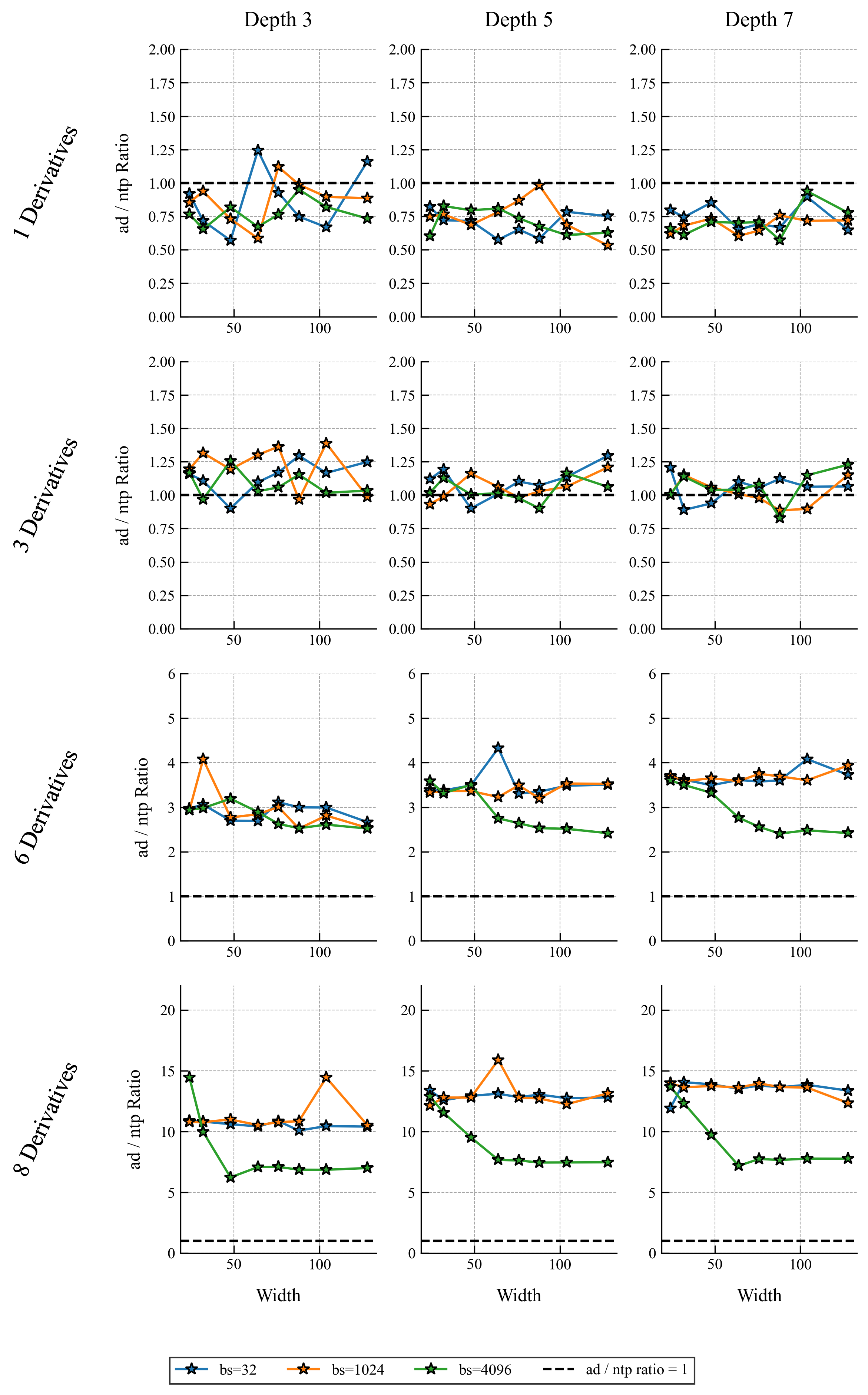
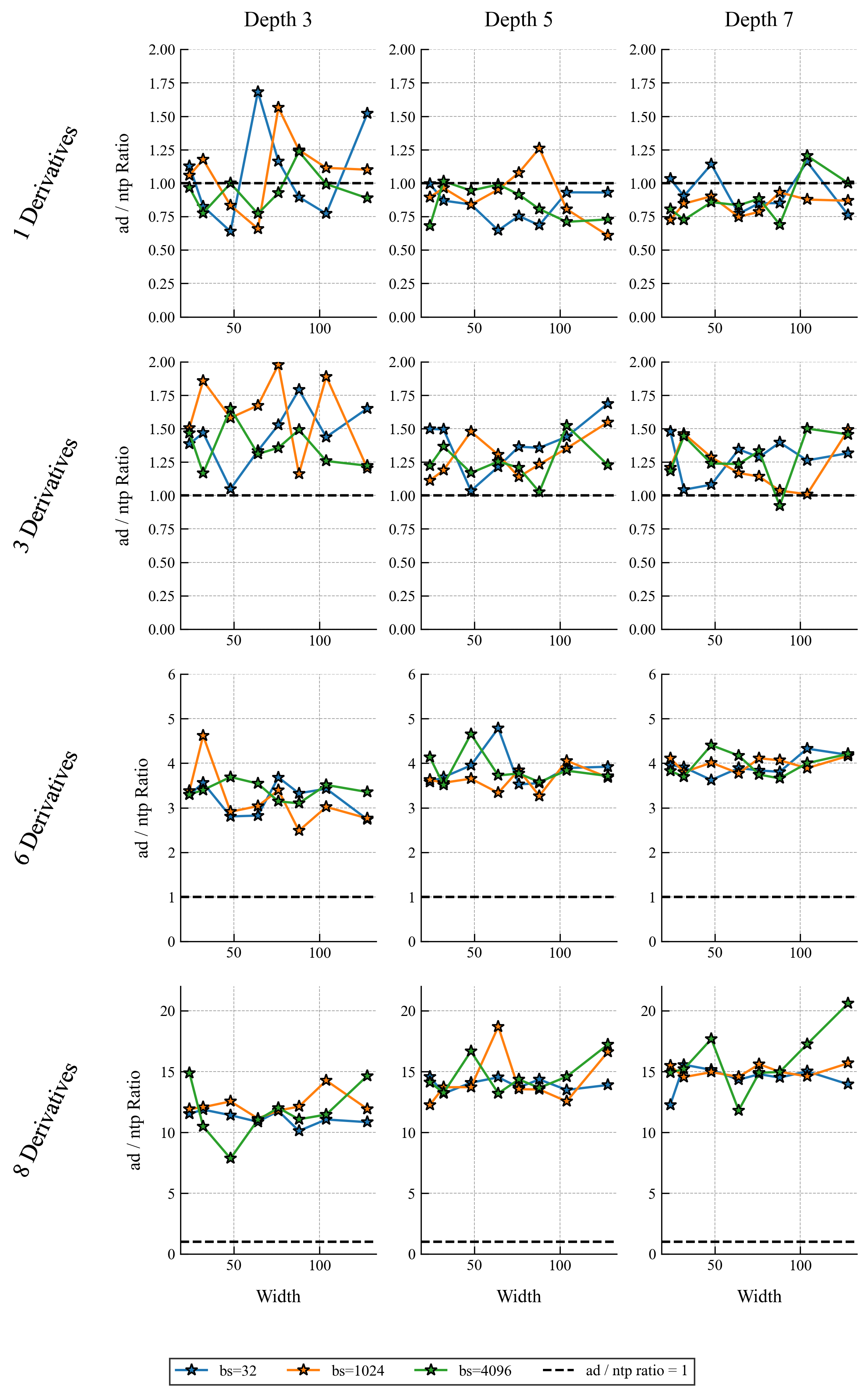
The following plots show the speed comparisons for simple forward and backward passes through a network (i.e. not training yet).
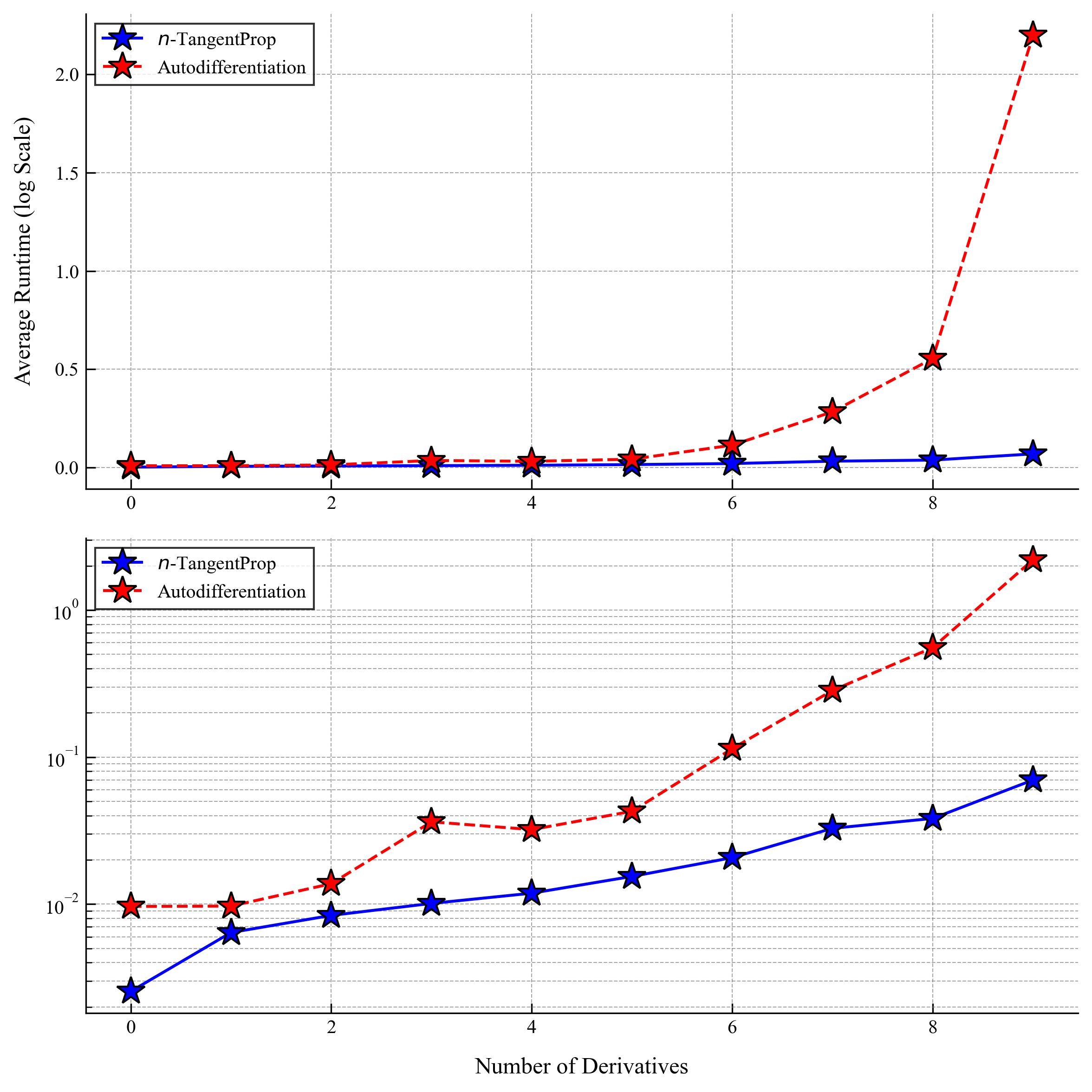
autodifferentiation (red) and -TangentProp (blue). The top and bottom frames show the same data, however the bottom frame is plotted with a logarithmic -axis. Each model is run 100 times and the average for each trial is plotted. The network has 3 hidden layers of 24 neurons each, a common PINN architecture. The batch size is samples.
Results for a Model Problem
To illustrate our method in a “real-world” application we consider the problem of finding smooth self-similar solution to Burgers equation. Burgers equation is the canonical model for 1D shock formation and is given by the PDE
One way to analyze shock solutions is to convert this equation into self-similar coordinates via the transformation
Under this change of coordinates the PDE becomes an ODE
with the scalar valued parameter .
This problem is not difficult to solve. It is an “advanced” exercise in an undergraduate course on differential equations and is solved by the implicit formula
However the numerical techniques developed to solve this problem can be applied to much more complicated and challenging problems for which implicit formulas for the solution do not exist.
To this end, we follow Wang et al. and deploy a PINN to solve this problem. A PINN is preferable here to a line search over since gradient descent will find both and simultaneously. Furthermore, is determined by a smoothness constraint at the origin and since PINNs are automatically , evaluating high-order derivatives at the origin becomes easy to implement.
.png)
.png)
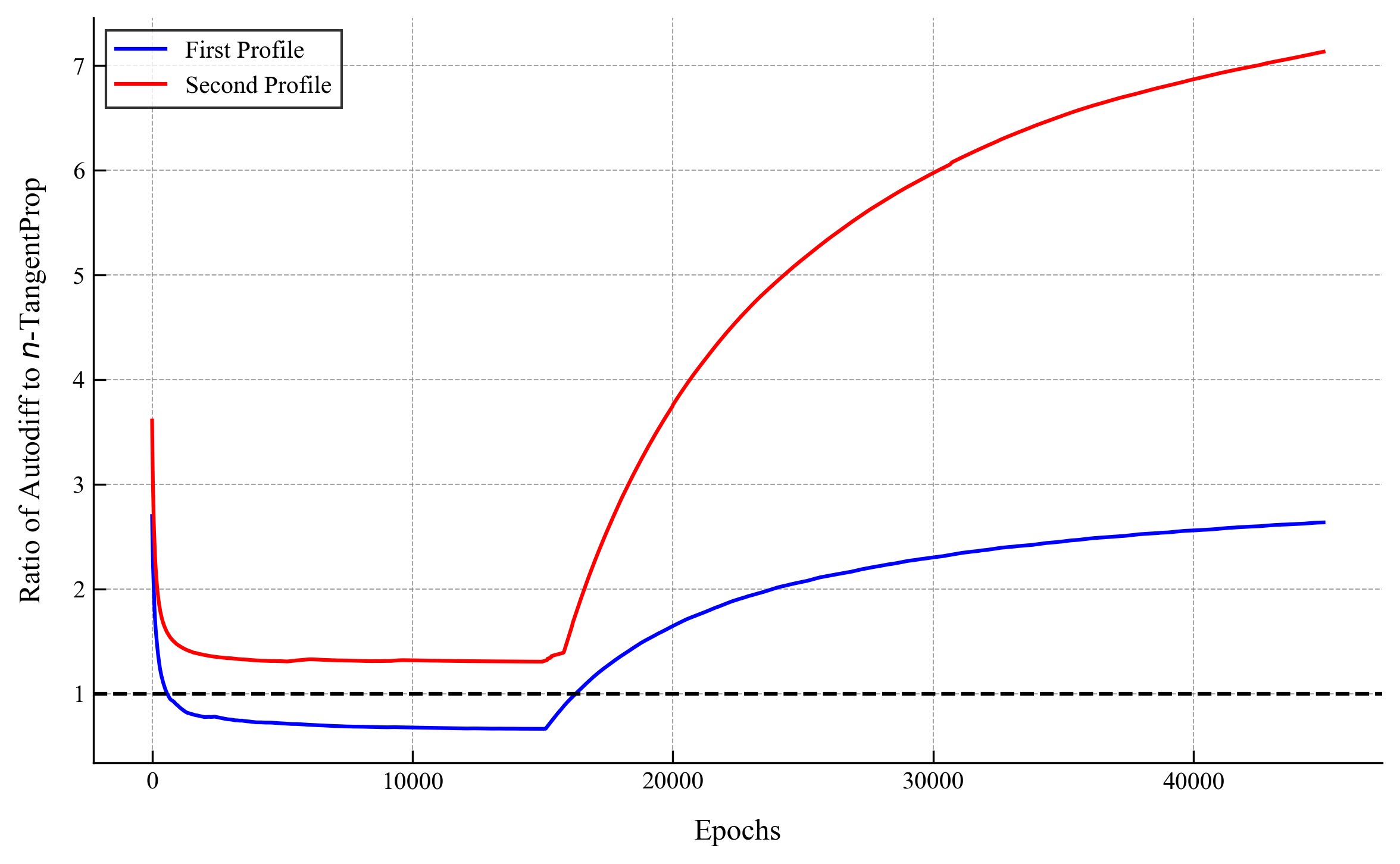
We observe that the widespread use of L-BFGS amplifies the benefits afforded by -TangentProp because the L-BFGS algorithm runs many forward passes but only a single backwards pass. As we saw in the previous section of our results, the gains afforded by -TangnetProp are more significant for forward pass than for backwards passes. Thus we see from above that during L-BFGS cycles -TangentProp begins vastly outperforming autodiff.
We only computed the first two profiles using autodiff. The reason is that already for computing the third profile using autodiff we needed more than 24 hours of compute time on an A6000 GPU, which went beyond our allowable compute budget. With -TangentProp this profile took a little under 1 hour, meaning that we had a speed up of over 24x. For the fourth profile we estimate that autodiff would take about 100 hours (around four days), and we were able to compute it on our computer in under an hour and a half, giving more than a 65x speed-up! Keep in mind that we only implemented minor optimizations for our code.
Conclusions
Based on our findings we recommend that any PINN use case requiring taking three or more derivatives implement -TangentProp to avoid needlessly wasting compute.
Consequences of this line of research include:
- Democratization of PINN research by allowing researchers without access to high-compute to study PINN problems.
- Enabling new avenues of study which require taking high-order derivatives of PINNs. In particular we can easily enforce smoothness and thus compute previously unknown unstable self-similar solutions.
- Providing more accurate solutions with less compute. By enabling more rapid computation of high-order derivatives we can now enforce successively higher Sobolev losses which will lead to more accurate PINN solvers.
Future Directions
There are several key directions that we could take this work in the future. I am not sure if I will take up the challenge, but if anyone is interested in these as projects please reach out and I am happy to help guide your work.
Of particular interest to me are the following two extensions:
- Optimizations: We did not optimize our code, there are many low-hanging optimizations that have to do with the graph, writing the forward procedure in C++, and using more of PyTorch’s built in optimization tools. Additionally we can implement low-level register and math operation optimizations to gain as much of an advantage as possible.
- Multiprop: We restricted ourselves to computing scalar derivatives in this work, but we can extend the work to encompass taking other derivatives as well. For example, we can compute the diagonal of the Hessian with respect to the weights in linear time! There are many interesting applications of our work in situations which require a sparse subset of a high-order derivative tensor to be computed. (I.e. computing the Laplacian on ).
About the author: Kyle R. Chickering is a PhD student in the department of mathematics at UC Davis. He holds a BS and MS in applied mathematics from UC Davis, and has worked in analytic shock formation, numerical methods using machine learning, and more recently, on large vision-language models. Outside of academia he has worked on teams building generative AI for video and has focused on efficient algorithms for machine learning. He lives with his wife, two dogs, and their cat in Davis, CA.
